Identifying different customer types with set expressions in FastStats

Introduction

This blog will discuss a group of analytical questions and show marketing use cases which were previously difficult to solve using FastStats. We shall review some basic ideas in set theory and show how the introduction of a set data type in expressions can allow us to identify interesting customer behaviour on the example of holiday booking data. I’ll also use this technique to investigate questions in football analytics that may well have never been asked before.

Differentiating between customer types

We will use one of our standard demo data sets including holiday booking data to illustrate the ideas in this blog post. This data contains information on our customers and the holiday bookings they have made (destination visited, booking date and cost information).

Holidaymakers have all sorts of preferences with regards to the destinations they choose to go on holiday to. Some people will revisit the same places, maybe even at the same time, every year without fail and don’t want to go somewhere new. Other people may never choose to return to the same place twice. The marketing strategies for these types of customers are very different. You may want to send messages relevant to one particular destination to customers you know who are returning there regularly. If you start promoting a holiday to a new destination, then it is probably sensible to send this information to people who regularly like going to new destinations. Further, you may also want to analyse the similarities or differences between each of these customer types using cubes or profiles. In this blog, we will look at how to identify people from these (and other) types using the so-called ‘sets expressions’ feature in our data analysis software FastStats.

Set theory

Sets are a standard mathematical concept that can help us answer many of the questions described in the previous section. This is not intended to be a full introduction to sets, and if you need to refresh your understanding of this topic, then there are plenty of resources online to understand some of the concepts that I am using here.

A set is a collection of things where each item only appears once. These can typically be any objects, but we shall be using them in this blog post where they are representing numeric values. So, for example it could be, Set S1 = {2, 3, 4}.

There are a number of standard mathematical operations on sets, for example here are two of them:

a)    Intersection – If S1 = {2,3,4} and S2 = {4,5,6} then S1 n S2 = {4} because this is the only item in both sets.
b)    Disjoint Sets – If S1 = {2,3,4} and S2 = {5,6,7} then S1 and S2 are disjoint because they have no items in common. 

Some of these operations will give the result as a set, others will return logical (True/False) or numeric values. If we imagine that the two sets above represented holiday destinations, I visited in year 1 and holiday destinations I visited in year 2 respectively, then there are clear marketing analytical use cases for the two functions above – namely ‘find destinations visited in both years?’, and ‘did I visit any destinations in both years?’.

Building sets in FastStats

In this development in the expression tool, a user can now use the ‘Create Set‘ function that can take parameters that consist of numerical values taken from the following possible list:

a)    A single numeric value
b)    A selector – the index of the selected value is added to the set (e.g. my occupation value)
c)    A flag array – the index of all the selected values are added to the set (e.g. values representing all the destinations I’ve visited)
d)    A list of numeric values (returned by one of the existing list functions)
e)    A set of numeric values (returned by one of the new set functions)

Once a set has been created, it can be used as a parameter in any of the set functions that have been added to the expression tool. The majority of these set functions are the standard mathematical set functions that you would hopefully expect to see. The results of these functions can then be used as input to other functions. The expressions can then be used in selections, viewed in data grids or used in cubes.

There are also a number of utility functions to work with sets, such as ‘Str Set’ to turn the set into a string, ‘Set Contains’ to test whether a particular value is in the set and ‘Count Set’ to count the number of items in a set.

Holiday customer example

In this dataset, I have customer holidays up to and including 2016. In this example, I will use holiday bookings from 2015 and 2016 for my analysis and look at identifying different customer types using set expressions.

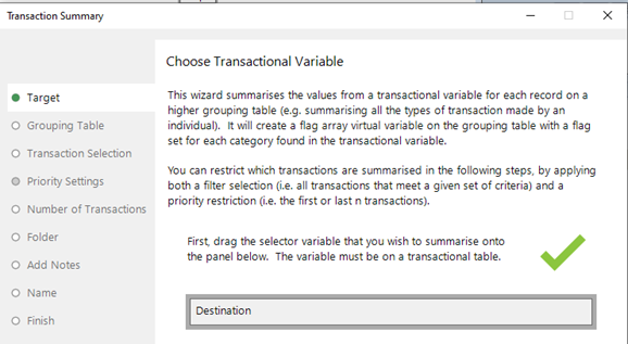
The first step in my analysis is to create a flag array variable for 2015 bookings and 2016 bookings so that we know which destinations have been visited in each year. We can do this using the ‘Transaction Summary’ wizard.

We then have two flag array virtual variables, as shown in the data sample below:

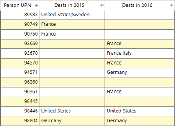
With a simple selection, we can find that 510,753 people had a holiday in 2015 OR 2016. Let’s segment those customers into some interesting groups using the set functionality.

As in the screenshot above, there will be many of those people who only holidayed in one of those two years, so we can look to identify them first. It is easy to make this as a selection without using sets, but we could also use sets expressions to identify these people using the following expressions:

a) 220,134 had a holiday in 2015 but NOT in 2016

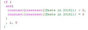
b) 213,126 had a holiday in 2016 but NOT in 2015

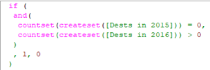
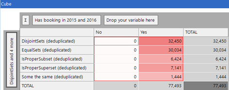
This gives a total of 433,260 people. This therefore leaves 77,493 people who have had a holiday in 2015 AND 2016, which we can then look at further. These can be broken down into these possible cases:

c) 30,034 had the same destination(s) in 2015 and 2016 (using the ‘Equal Sets’ function)

d) 32,450 had entirely different destinations in 2015 and 2016 (using the ‘Disjoint Sets’ function)

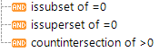
e) 15,009 had some common destinations (Intersection sets non-empty AND not equal sets)

If we add up each of these three cases, we find that the total is 30,034 + 32,450 + 15,009 = 77,493 people. We have identified all the people, but those with some intersection can be split down further as follows:

e1) 7,141 had all from 2016 in 2015 (superset) [e.g. destination of 2015 AB, 2016 A]

e2) 6,424 had all of 2015 in 2016 (subset) [e.g. destinations of 2015 A, 2016 AB]

e3) 1,444 have some destinations the same but are not (e1) or (e2) [e.g. destinations of AC, BA]

We can see all of these on a cube – as below.

Each of these different variations highlights a different type of customer that we may want to analyse, or use for campaign activity, as described in the earlier section. We could have created further sets to identify behaviours over multiple years for example.

More involved examples

In many previous blogs, we have tested new FastStats functionality on our football system (see for example my blogs on ‘Sequencing transactions with pattern matching’) to find interesting insights from international or English league football. This system contains data on all the English league football matches up to the end of the last completed season (2020-21 season).

Here are a couple of questions that we can look to answer with the sets functionality. 

1. How many English league teams have recorded the same set of scorelines in the last two seasons? (2019-20 and 2020-21)
2. Has any team ever recorded the same set of scorelines in any two seasons since WW2?

Using the same technique as we outlined earlier, we can firstly create variables using the ‘Transaction Summary’ wizard to create a flag array of the different scorelines achieved during those particular seasons. In the screenshot below, variable ‘ELS2019’ is such a flag array.

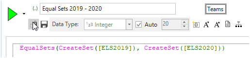
We could then use the expression below to return if the two are the same:

If we then show a data grid of all the teams that have played in 2019 and 2020, a part of the grid is shown below.

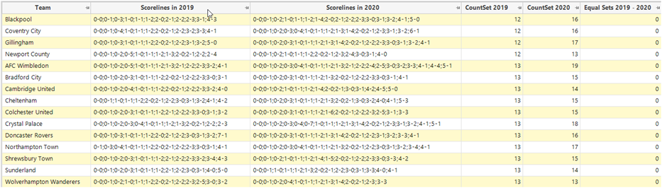
There are no positive results in the final column, but we can dig into those results a little further to see how similar two of them are.

Bradford City’s scorelines in 2019 are a subset of those in 2020.

Salford City’s scorelines in 2020 are a subset of those in 2019.

Finally, if we consider the number of different scorelines in a season, we would find that there were 12 teams who had the same number of scorelines in each season.

Is this normal or abnormal to have no common set of scorelines? (see note 1 at the end for a lengthy discussion which concludes that this would be unlikely!!).

Now let’s consider a much more general question: 

“In the 75 seasons since WW2 - how many times has a team had any two of those seasons in which they have recorded the same set of scorelines”?

A) This has happened only twice since WW2, namely Wolves (1969 and 2007) and Aston Villa (2006 and 2016).

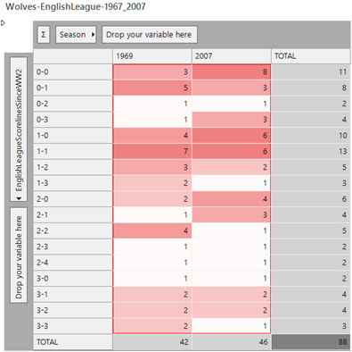
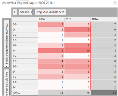
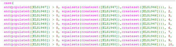
This has been achieved by creating a variable for each of the 75 seasons and then constructing an expression as below. Each line checks that there are some results in the first season, and also that the pair of seasons has the same set of scorelines. There are 2,775 lines to the expression for all of the (75 * 74 / 2) possible pairs of seasons. The result of the expression will either be 0 (there are no matching pairs of seasons for the team) or the number corresponding to the first pair of seasons in which this has happened [Note – by removing the matched values and rerunning the analysis, we can prove that these are the only two such occurrences!!].

Further work…

As a final piece of analysis, we adapted the table structure of the system to enable us to look for common scoreline sets between team/season combinations. We can use this to find out for instance the most common scoreline set across every team/season combination in the English League. The screenshot below shows that there are a number of scoreline sets that have occurred 6 times. The highlighted one has been achieved by 5 different teams, and if we drill into those, we can see the Aston Villa combination from earlier as well as 4 other instances from other teams. 

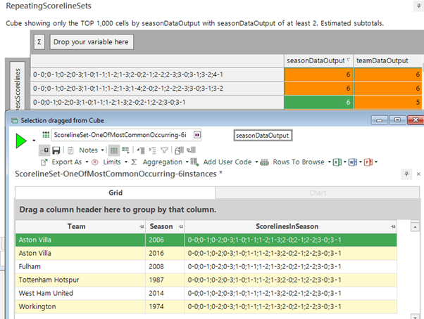
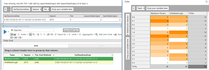
And, as a final insight if we add season and tier (Premier League, Championship, League 1, League 2) to the analysis (top left of screenshot below) we can see that there is only one instance where a scoreline set has been registered by the same team in the same season in the same division. We can see which two teams in the bottom left, and then the cube on the right shows the individual match scorelines for those two teams in that season – and we can verify that the sets are indeed the same.

Conclusion

The introduction of the idea of sets within expressions has given FastStats the ability to answer a range of analytic questions either more simply than before, or in some cases even at all! The functions which act on these sets are mathematically well known in almost all cases. 

The limitations in the above examples are primarily around the need to often create a new variable using the ‘Transaction Summary’ wizard. For more significant scenarios such as the football example, this can involve having to create a large number of variables before the analysis can take place. This can be time-consuming, prone to mistakes and leave a large number of variables in the system which don’t get used again. Furthermore, any slight change to the requirements of the analytics could mean having to edit those variables to change definitions or create a new lot of variables. In some scenarios, the grouping aggregation developments described in this blog will mean that for scenarios where sets are based on a single variable, we can get around this step without needing to create any variables.

 

General considerations:

A team has 38, 42 or 46 matches in any season. Clearly, they can then have a different number of scorelines in any season - but generally we find that it is in the range of 15-20. There have been 100 different scorelines achieved in English league football since WW2, but a significant number of these have only been achieved occasionally - there are maybe 25 to 30 that have happened a reasonable number of times. 

Assuming each team achieves 16 different scorelines every season out of the 25 most common, there are C(25, 16) = 2,042,975 different sets of scorelines possible for a given season. There is potential for things to get confusing here as we’re dealing with things that themselves are sets, but it’s better to try to forget that and just think of each of these sets as a single entity – a “scoreline set” – and that we have a “pool” of these. Each team in each season will have exactly one of these objects “assigned” to them. 

1. Probability of any team recording the same set of scorelines in the last two seasons 

Begin by calculating the probability of a specific team recording the same set of scorelines: once they’ve played the first season, the scoreline set for that season is fixed so they have a 1/n chance of “picking” the same scoreline set for the second season (where n is the number of different possible scorelines). So, this is 1/2042975 ≈ 0.0000489% 

To calculate the chance of any team recording the same set of scorelines, it is easier to calculate the opposite first: the probability of no team recording the same set of scorelines, i.e. every team recording a different set of scorelines. For one team to record a different set of scorelines is the complement of the above calculation: 1-1/n = (n-1)/n or in our case 2042974/2042975 ≈ 99.999951% 

For every team (and there are 90/91 who will have been present in both seasons because of promotion and relegation, so t = 90/91 in our calculations), to record a different of scorelines is then this figure multiplied together once for each team, i.e. [(n-1)/n]^t which gives 99.9956%. 
So, the probability of any team recording a repeated set of scorelines is the complement of this: 0.0044% 

P(any team records same set of scorelines in last two seasons)
= 1 – P(every team records different set of scorelines in last two seasons)
= 1 – [P(one team records different set of scorelines in last two seasons)]^t

P(team records different set of scorelines in last two seasons)
1 – P(team records same set of scorelines in last two seasons)
= 1 – 1/n

P(any team records same set of scorelines in last two seasons) = 1 – (1 – 1/n)^t

2. Probability of any team recording the same set of scorelines in any two seasons since WW2

As before, we begin by calculating the probability of this occurring for a single team. There have been 75 seasons since WW2, so we need the probability of having a repeated set of scorelines among 75 sets (one set per season) “picked” from 2,042,975 (the n we calculated above). Again, it is easier to calculate the complement of this: the probability of no repeated scoreline set, i.e. the probability of 75 different scoreline sets when picking from a total pool of 2,042,975 scoreline sets. 

To make it easier to understand the calculation, imagine an example with simpler numbers: picking 4 objects from a pool of 10 possible ones, and considering what happens as we pick them one-by-one.

The chance of the first object being unique is 1 since we haven’t picked anything else yet. For the second object to be unique we need to pick one of the 9 remaining not-yet-picked objects out of the 10; for the third object to be unique we have an 8 in 10 chance of picking an object that hasn’t been chosen already, and so on. So, the overall chance of all 4 being unique is: 1 × 9/10 × 8/10 × 7/10. For consistency we can think of the initial 1 as being a choice of any of the 10 objects from the initial 10, so we can also write this as: 10/10 × 9/10 × 8/10 × 7/10. 

The same idea applies to our situation, so the probability of a team having no repeated scoreline sets is: 2,042,975/2,042,975 × 2,042,974/2,042,975 × 2,042,973/2,042,975 × …  × 2,042,901/2,042,975 ≈ 0.998643.

(This calculation can also be approximated as exp(-C(k, 2)/n). In our case n = 2,042,975 and k = 75)

The probability of none of the teams having a repeated scoreline set is then this multiplied by itself for each team: 0.998643^92 ≈ 0.882527. So, the probability of at least one team having at least one repeated scoreline set is the complement of this: 0.117473 = 11.7473%.

P(any team records same set of scorelines in any two seasons since WW2) 
= 1 – P(no team records same set of scorelines in any two seasons since WW2) 

P(no team records same set of scorelines in any two seasons since WW2) 
= P(every team records different set of scorelines in every season since WW2)
= [P(one team records different set of scorelines in every season since WW2)]^t 

P(one team records different set of scorelines in every season since WW2)
= n/n × (n-1)/n × (n-2)/n × … × (n-74)/n

P(any team records same set of scorelines in any two seasons since WW2) = 
1 – [n/n × (n-1)/n × (n-2)/n × … × (n-74)/n]^t

Further considerations:

The final answer of about 12% suggests this is quite a rare occurrence, about a 1 in 8 chance. If we looked at the comparable football leagues for 8 countries since WW2, we’d expect it to occur once. But as we’ve seen, there are several occurrences of this even just within the English football league, which suggests our calculations might be a bit off the mark. 

The key figure in these calculations is n, that is, how big the pool of different sets of scorelines is. We calculated this by assuming that every set (every team’s season) has 16 different scorelines from a possible 25, giving C(25, 16) = 2,042,975 possible scorelines. However, there are other assumptions and calculations we could have done here. 

While 16 is the average number of different scorelines in a team’s season, only a proportion of the seasons have this exact number. A range of 15 to 19, however, covers the vast majority of scoreline sets. Including scoreline sets with this number of different scorelines, gives us: n = C(25, 15) + C(25, 16) + C(25, 17) + C(25, 18) + C(25, 19) = 7,104,240. This brings our final answer down to a probability of just 3.56%. 

One key assumption we’ve made is that each scoreline is equally likely to occur, but we know this is definitely not the case in reality. There are some scorelines which nearly every team records in nearly every season; the most common being a 1-1 draw. It would require quite complicated calculations to introduce some kind of weighting system for different scores, but we could change our assumptions when calculating n to try to account for this in some way. If we assume that every team is guaranteed to record the 5 most common scorelines (e.g. 1-1, 1-0, 0-1, 0-0, 2-1) we can “pre-allocate” these to every season, which leaves 10-14 other scorelines to pick from the remaining 20: 
n = C(20, 10) + C(20, 11) + C(20, 12) + C(20, 13) + C(20, 14) = 610,470. This brings our final answer up to 34.9%. 

Similarly, assuming 6 given scorelines gives 53.0% and 7 takes us up to 74.6%. 

Another factor we could consider is the role of outlier scorelines. If a team has a particularly unusual scoreline (one where one or both teams score a high number of goals) that occurs very rarely, that is likely to be enough to guarantee that their scoreline set for that season will be unique; it’s unlikely one of the other rare occurrences of that scoreline also happened in one of their seasons and that the rest of the scorelines from that season also matched. Depending on how many seasons have an outlier scoreline, we might write off a proportion of the seasons before we even start – perhaps leaving only 50 or 60 to consider in our calculations, rather than 75.