Step into the map - The latest developments in thematic mapping

7 min read

Maps are a well-used analytical tool that enables users to derive insight from location-based data.

A standard way of visualising this information is through a choropleth (or thematic, or shaded) map. This type of map comprises a number of shapes that represent related locations which are coloured in such a way to represent a quantity where the colours are on a shaded scale that indicates bigger or smaller values. An example of insight that could be gained from these types of maps might be ‘our better customers are located in the South’.

In FastStats, we have always supplied a standard set of postal-based shape files for thematic maps as our clients are usually working with customers who have physical delivery addresses. Breaking these down into postal areas for example is quite a natural way of visualising this information.

It has always been possible to incorporate your own shape files but this has always required specialist skills and behind-the-scenes access in order to configure the system to allow for customised maps.

In this blog, we will show new developments in FastStats that make it much easier for the end-user to build thematic maps from shape files directly.

Standard shapefile mapping – Linking to existing variables

In a previous blog post (see Note 1) we analysed data from police reports on UK traffic accidents. Map visualisations on this data using our standard shapefiles would have been impossible as there were no postal variables defined in the source data. Furthermore, accidents wouldn’t naturally fit into this type of data as a sensible unit for analysis by. Each accident did contain latitude and longitude information to give its exact location so a user could produce plot maps of say locations of significant accidents, but the granularity of the produced map would mean that it couldn’t provide insight into good overall trends within the data. Finally, it couldn’t be used to look at visualisations at police force level (e.g. what is the average number of vehicles involved in accidents by Police region – but visualised on a map).

Each accident record was also attributed to the police force responsible for it, and each of those forces have a particular geographical area of operation. Being able to analyse and furthermore visualise that information is valuable. However, FastStats does not come with pre-configured shapefiles for ‘police force area’ in it.

The ONS boundary files website (Office of National Statistics, Open Geography Portal (statistics.gov.uk)) curates a wide range of useful geographical shapefiles from a range of different domain areas (administrative, health, political amongst others). Within this they have available shapefiles in multiple formats that represent police force areas.

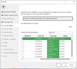
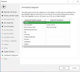
Linking a shapefile to an existing variable in a FastStats system is now straightforward. In the Territories wizard we specify the shape file and the feature within the file that contains the ‘names’ of each of the shapes within it. Any discrepancies between the categories in the variable and the shapefile (e.g. spelling differences) are then flagged up for the user to match them up. In the screenshots below the user chooses the name field from the shapefile and then resolves any unmatched variable categories to the names in the shapefile. In this example, the system contains Scottish data, but the shapefile only covers England, so there are some categories which needed linking up, and others which cannot be visualised using this shapefile.

Then the user can drag the variable onto the map and see the breakdown of it.

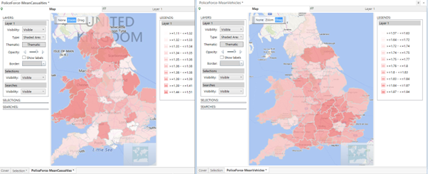
Also within the data is information on casualties and vehicles involved in the accidents. Using the Mean (Number of Casualties) and Mean (Number of Vehicles) as the thematic statistics and plotting by police force area allow us to see if there any interesting geographic relationships between these variables.

From the right-hand panel we can see that there are a higher number of vehicles involved in accidents in areas with dense populations and larger motorway networks. From the left-hand panel we can see that the areas with higher numbers of casualties tend to be areas covered by more rural police forces.

Standard shapefile mapping – to a new variable

There will be many instances where we have precise location information for the customer (or data record), and we would like to produce a thematic map but the data does not contain a variable that identifies which shape a customer belongs in.

In the example below, I have some customers from a German system. I have data that contains their latitude and longitudes, and a shapefile for federal states, but would like a Selector variable showing which of these each customer belongs to.

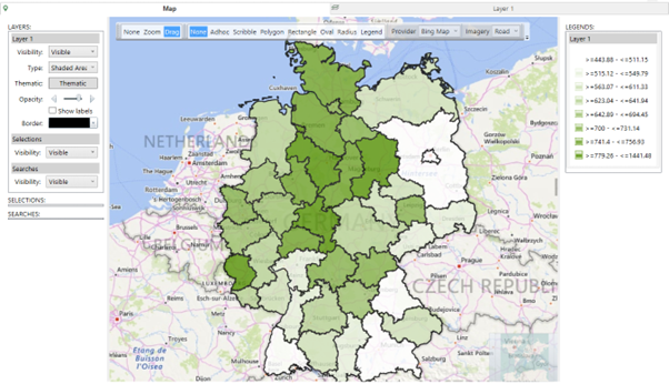
The territories wizard now can undertake this allocation process and create that variable, whilst simultaneously creating a version of that shapefile that can then be used as the basis for displaying thematic maps. In the example below, for each state we are showing an average holiday cost for the customers who live in each of these states.

DriveZone Mapping

FastStats has long been able to do analysis by drivetimes from locations to produce variables. These centre points are often store locations. The zones could represent customers within 15, 30, 45, 60 minutes drivetime of that location. Users could then use this information in selections or produce analysis using cubes showing metrics broken down by customers at different drivezones from these points.

However, until now they have not been able to visualise those metrics or the extents of those drivezones on the map tool. A single extra checkbox on the wizard will then create the associated shapefile representing the extents of each zone whilst the variable is being created.

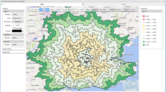
This first example has a single location of interest (Heathrow Airport), and each zone is a 10 minute zone up to a time of 2 hours from Heathrow. The shape boundaries clearly demonstrate the main routes radiating out from the M25 as these enable customers to travel further. In this screenshot, we are looking at the average holiday cost value for customers in each of these drivezones around the airport. I’ve used a custom colouring scheme that highlights the green ones as having higher value and the darkness of those colours that suggests that there might be a relationship between travel time to the airport and the average holiday cost.

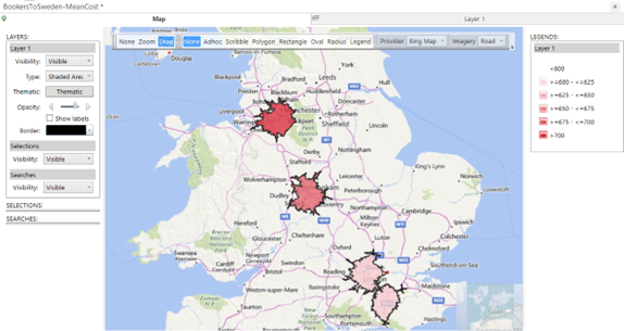
In this second example, our imaginary Holidays company is interested in the number of customers of theirs within 30 minutes drivetime of each of their locations of interest which are four of the major UK airports. This is a single layer map of a flag array variable (since there is an overlap between the 30-minute Gatwick and Heathrow zones). It is suggesting that the average holiday cost of customers around the Northern airports is higher than the Southern airports.

Case study – Political party mapping

For a final example, I’m going to use FastStats to replicate map visualisations which are often seen on TV election coverage. I have created a very small dataset from the 650 Westminster Parliamentary constituencies that simply has the votes recorded for each party, the winning party and some electorate details for each constituency record.

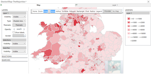
The ONS provides a shapefile for parliamentary constituencies which can be linked to the constituency name and any differences ironed out using the technique described earlier. There are a number of interesting ways in which we can colour this map. One way would be to shade each constituency by the majority to see if there is any interesting geographical basis to where the election battlegrounds will be at the next election. In the screenshot below, the darker reds are highlighting the constituencies with smaller majorities.

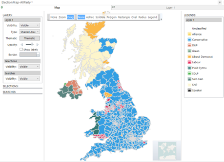
However, we can also colour this map using a customised colour scheme. One such example would be to colour each constituency by a colour that is representative of each political party. The map below shows this in action. I have linked the colours to the values of a metric of the winning party that then shows the concentration of Labour seats in urban areas around London, Birmingham, Manchester and the South Wales valleys and the huge tracts of more rural seats across the south of the country that are represented by Conservative MPs. The legend on the right has been customised so that rather than showing a numeric value it shows a more representative textual value for the colour.

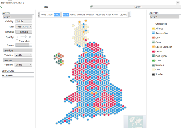
One weakness of the above visualisation is that in this particular example each geographical seat has an equal weight interpretation (they each send 1 MP to parliament). However, the larger geographical area of the Conservative seats means that our first reaction is that there must have been a huge majority. An abstract shapefile with equal sizes for each constituency laid out in such a way to try and best preserve the geographical representation can help in these instances, although they have to make simplifications on how to map the original shapes to the hexagons.  The example below shows the same data as above but utilises a shapefile that represents each constituency as a hexagon. It clearly shows that there are more Labour MPs than we imagined when we saw the first visualisation.

This dataset utilised the Parliamentary constituency shapefile to simply link to the variable. However, if you wanted to work out which constituency each of your customers belonged to then the territories wizard (using the technique from the German example earlier) applied to that data would produce a selector variable indicating which constituency each customer belonged to that could then be visualised using that shapefile (this needs to use the actual geographical version and not the hexagonal one!).

Conclusion

This blog has shown that we can classify our customers, or data points, into which shape they belong to and then generate maps on those metrics. The generality of the technique means that we can use standard shapefiles from different sectors (e.g. political, healthcare etc), or customised one based on useful marketing analytical location results such as drivetime.

References

Note 1 – A previous blog post on UK Traffic accidents (Have UK roads become safer in the past 40 years? | Apteco)