Sequencing transactions through pattern matching – part 4

Introduction

In previous blog posts (see parts 1, 2 and 3) we introduced the idea of pattern matching as a way of understanding sequences of transactions for a customer. This powerful technique can be used to both select from, and analyse a customer database and provide insight into interesting transactional behaviour.

In our previous blog posts, the algorithm returned a single value representing matches on the grouping table. There are cases when returning a value on the transactional table for every transaction can enable us to get a better understanding of the particular type of customer each person is.

In this blog, we illustrate some of the analytical questions that we can now seek to answer. We also revisit football analytics to answer the all-important question about which team really have the fans that have to put up with the most suffering!

Understanding subtleties in transactional behaviour

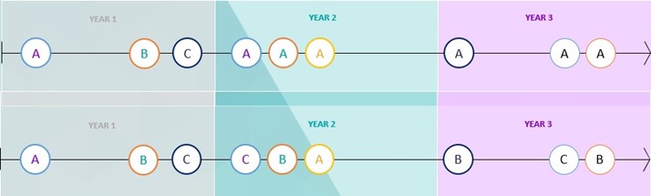
In the screenshot below there are two people who both have the same number of transactions, but it is clear after quick inspection that the two people have very different holidaying behaviour. Person 1 has started with three different destinations, before settling back to going to the same destination repeatedly. Person 2 has the same initial three transactions and then switches between the three destinations.

If we look for a person’s propensity to switch holiday destinations, we might look for the length of sequences of entirely different holiday destinations. We can use a set of patterns like this:

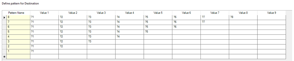
This will be a sufficient number of patterns on our Holidays system because I know that the maximum number of transactions a person has had is 8.

For each of these two people, they would return the same value on the person table – their longest sequence of different destinations is 3. In both cases, this equates to the first 3 transactions for each person. By this metric, Pattern Match will think that these two people are the same.

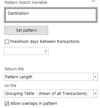
In this new development, we can return the value on the child table. For each transactional value, we return the highest priority pattern that starts at that transaction. If no pattern starts at a given transaction, then no value is returned for that transaction.

In the Pattern Match definition, we then take the mean length of the pattern above across all of the transactions.

For our example above, this set of patterns is sufficient to return a value for every single transaction, as shown in the diagram below:

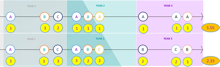
The average across all the transactions is shown in the orange ellipse on the right. We can then use this expression as a measure on a cube. In the example chart below, we have broken down our customers by Income and we have also included a measure for the Mean (Number of Bookings) for each Income band.

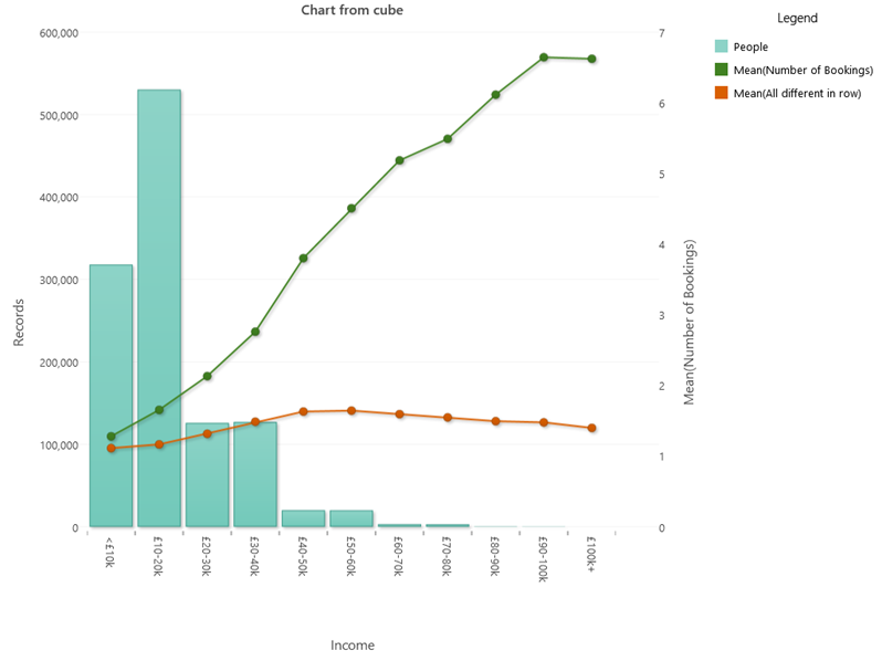
What insights do we get from the above example?

1. Most of our people are in the lower income bands and this drops off quite sharply, so we have few people to base our insights on in the upper income bands.
2. The average number of bookings has a definite relationship with the income band. The higher the income band the more holidays on average are taken.
3. The orange measure (which is our propensity to switch measure from above), however, shows that average length of different holiday destinations rises until the middle income bands and then falls away in the higher income bands. There are two important aspects here:

• With a low number of bookings, you can only have a low value since you don’t have the chance to build up a long sequence of different ones. For a person with 1 booking, they will have the value 1. For a person with 2 bookings, they will have a value of either 1 or 1.5.
• In the higher income bands the value of the pattern match measure is smaller which suggests that these people tend to visit the same holiday destinations regularly. This is an interesting insight!

We could also have used this metric as a way of selecting records – for example selecting the top 10% of my customers who are likely to switch destinations – and this could be used as a good target for promoting a new holiday destination recently added to our brochure.

Transaction sequences in football results 

I have used football results in many of my previous pattern match blog posts, as this is a good example of data with a large number of transactions (matches) for each team. The data structure is Team->Match (i.e., a team has lots of matches). We can use the pattern match technique above to find teams that keep on repeating the same result type (winning or losing!), or who cycle through the different results (the very definition of supporting your team through thick and thin!)?

We can do this using the same technique as the holidays example above, but since a team can only have 3 possible results (Win, Loss, Draw) before repeating one of them, we only need to use ?3?2?1 as the longest sequence of different results. A team that is always repeating the same results will have an average difference length of 1, and a team cycling through all possible results in the same order will have an average difference length of 3.

Let us consider English league football on a season-by-season basis (3). In general, there are sequences of 38 to 46 matches depending on the season and the division a team was playing in. The pattern match aggregation in the expression is then used in the final statistic as a Mean to give the relevant figure for each season.

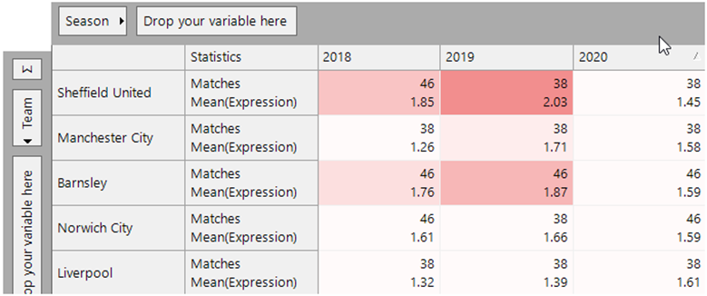
Our first view below is at the results for the last 3 completed league seasons, sorted so we can see the lowest scoring teams in the last season. Manchester City (lots of wins) score lowly as they have had less opportunities to switch result types. However, their score in 2020 of 1.58 was significantly higher than the 1.26 and 1.32 scored by them and Liverpool in 2018 in the title race that went down to the deciding day. Other teams such as Norwich and Sheffield United scored lowly by this metric as a result of losing a lot of games.

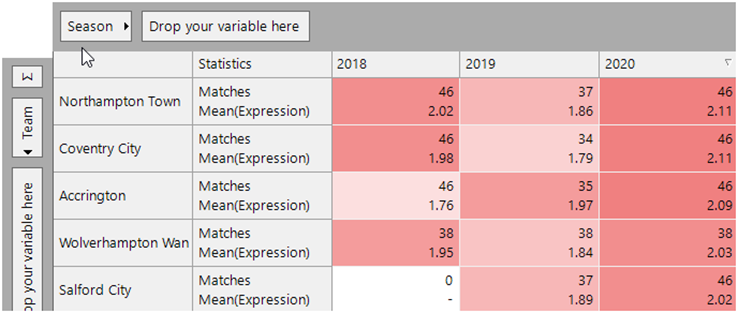
For a team to score highly by this metric they must have a similar number of results from each category and had few sequences of the same result – in the 2020 season Northampton (position 22 in league 1) and Coventry (position 16th in the Championship) satisfied these criteria.

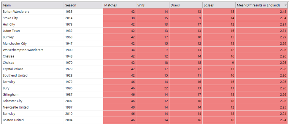
Let us now expand this out to look at the results across all seasons. How do these extreme scores (1.26 to 2.11) compare historically?

In each of the following pieces of analysis, I have added statistics to show the number of Wins/Draws/Losses in each season using query-based statistics. Firstly, looking at the highest scoring seasons, we can see that the 2.11 doesn’t even come close to the most mediocre of historic seasons! No team has come close to the 2.48 from Bolton Wanderers in 1935, but a very good effort by Stoke in 2014 sees them take second place on the list with an average of 2.34. 

Conversely, the all-time lower scoring seasons shows that the 2018 seasons of Liverpool and Manchester City are only beaten by Sunderland in 1891 (the rows are ordered here with the lowest scores at the bottom). The other interesting insight from this list is the number of seasons that are either in the last few years, or from over 100 years ago. This suggests that there were dominantly good or very bad teams in the early leagues, and then more recently we are seeing a similar pattern emerging of dominance or dreadfulness – especially in the Premier League, which suggests that the best players are being concentrated into fewer top teams.

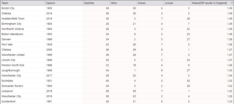
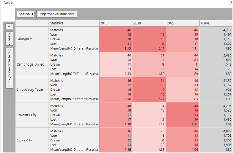
Finally – if we look at the whole history of a team’s English league matches then which team do we find has had the highest score? The list below is filtered to teams which have played at least 1000 league matches (roughly 25 seasons) and who have played a match in the 21st century. This was in order to ensure teams who are more current and who have played enough matches to remove statistical outliers. To the supporters of Gillingham, Cambridge, Shrewsbury, Coventry and Stoke, I salute you! 

Conclusions

This blog post has introduced functionality that was introduced in the Q1 2020 release. This new functionality allows the analyst to answer a wider range of pattern match questions and also to use the ability to return pattern values on the child table to understand more about the subtleties of patterns throughout a transaction history.

References 
1)    Previous blogs on pattern match analytics 
Sequencing transactions with pattern matching Part 1, Part 2, Part 3

2)    A quick note on the season-by-season calculations. The last 2 matches of each season allow the sequence to go beyond the end of the current season into the first match or two of the next season which gives a fairer season average than restricting the last 2 transactions down slightly.

If you would like to learn more about how to get the most from your data and stay ahead of your competitors download our eGuide.